Stock prediction
Quantitative analysis of certain variables and their correlation with stock price behaviour. This used to be hard, but now with powerful tools and libraries like tensorflow it is much simpler.
In the 1980’s two British statisticians, Box and Jenkins, created a mainframe program to attempt to predict stock prices from just two data points, price and volume. It was known as Autoregressive Integrated Moving Average (ARIMA).
The Box-Jenkins approach claims that non-stationary data can be made stationary by differencing the series, Yt :
Yt = Φ1Yt-1+Φ2Yt-2…ΦρYt-ρ+εt+θ1εt-1+θ2εt-2+…θqεt-q
The ARIMA model combines three basic methods:
- AutoRegression (AR) – Auto-regression, the values of a given time series data are regressed on their own lagged values, which is indicated by the “p” value in the model.
- Differencing (I-for Integrated) – Conversion of a non-stationary time series to a stationary one to remove time trends. This is indicated by the “d” value in the model. If d = 1, it looks at the difference between two time series entries, if d = 2 it looks at the differences of the differences obtained at d =1, and so forth.
- Moving Average (MA) – The moving average nature of the model is represented by the “q” value which is the number of lagged values of the error term.
A modern approach using artificial intelligence (AI)
The approach uses Keras, an API used to simplify prototyping on top of AI frameworks like Google’s Tensorflow. Google Tensorflow has its own flavour of Keras, which I use below with Python 3.6 to build a deep learning model.
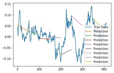
The very simple approach below uses only a single data point, the closing price with a deep neural network of only 2 layers using time sequence analysis recurrent networks variant LSTMs.
The code can be found at simple LSTM.
Data set
The data was from the daily closing prices from S&P 500 from Jan 2000 to Aug 2016. The series was indexed in time order.
Goal
The goal was to predict the closing price for any given date.
Output


